A Raytracer in Python - Part 3 - Samplers
In the previous post, we explored a very basic way of plotting images: shooting a ray from the center of every pixel, and plot the color of the object we hit. The result is a rather flat, very jagged image
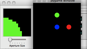
Border jagging arises from the fact that we are sampling with a discrete grid (our ViewPlane) an object that is smooth due to its functional expression (our spheres). The sampling is by nature approximated, and when mapped to pixels it produces either the color of the object, or the color of the background.
We would like to remove the jagged behavior. To achieve this, we could increase the resolution. That would make the jaggies less appreciable thanks to a higher number of pixels. An alternative is to keep the lower resolution, and shoot many rays per each pixels instead of only one (a technique called supersampling). To compute the final color, weighting is performed according to the number of rays that impact vs. the total number of rays sent from that pixel. This technique is known as anti-aliasing.
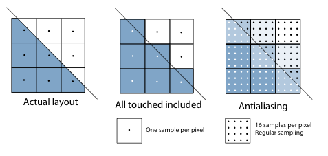
The figure details visually what said above: the real description of the sphere is smooth (left hand figure). Shooting one ray per pixel, and coloring the pixel according to hit/no-hit, produces either a fully colored pixel, or a fully background pixel (center). With supersampling, we shoot a higher number of rays, and per each pixel we perform weighting of the color.
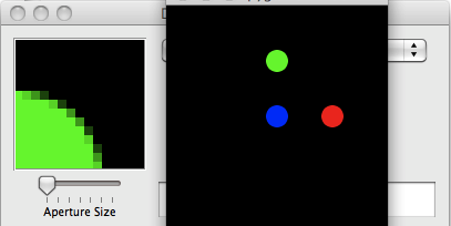
As a result, the jaggies in the sphere are replaced with a smoother, more pleasant transition
Choice of Samplers
The pattern used for the supersampled rays is important. The module samplers in the python raytracer implements three common strategies.
Regular sampling
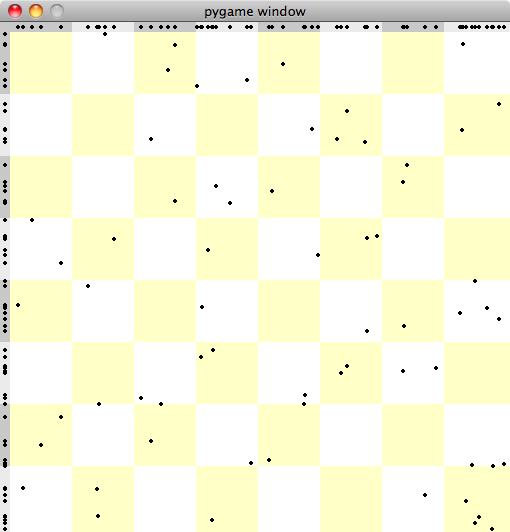
It is the most intuitive and easy, and the one used above: a regular grid of rays. It is easy to implement but it can introduce unpleasant artifacts for more complex situations. Plotting the position of the rays in the pixel will produce the following layout (for a 8x8 supersample grid)
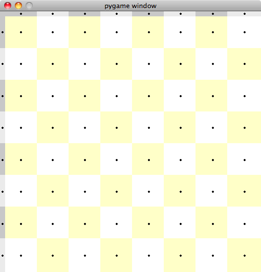
As we see, the layout is regular on the grid of subcells (painted yellow and white for better visualization) that define the pixel. On the vertical and horizontal distributions (plotted on the grey bars above and on the left) we also see a regular distribution, but its regularity may introduce artifacts in some cases.
Random sampling
Random sampling positions the rays at random within the pixel. This may sound appealing, but it may instead end up as suboptimal: it can produce random clumping, in particular for a small number of samples. This will unbalance the weighting leading to an incorrect evaluation. Plotting one distribution one may obtain
Note the uneven distribution of the points, leaving large parts not sampled and other parts oversampled. In addition, the vertical and horizontal distribution tend to be uneven.
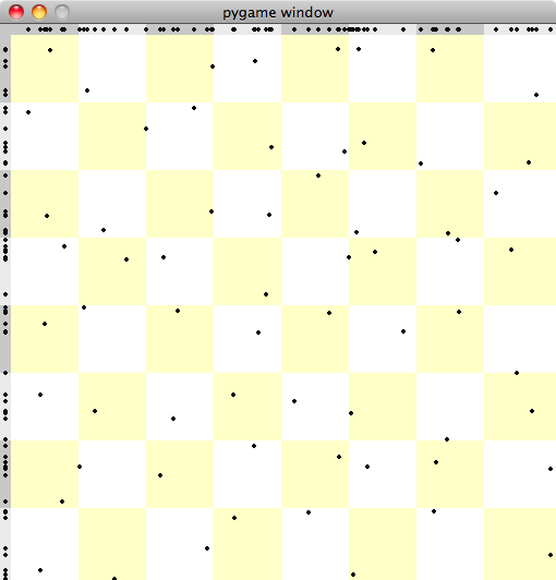
Jittered sampling
Jittered sampling takes the best of both worlds: the regularity of the Regular sampler with a degree of randomness from the Random sampler. The idea is to select the center of each subcell and apply randomization, so that each subcell produces only one ray, but without the artifact inducing regularity proper of the Regular sampler.
Computational cost impact
Unfortunately, performing supersampling makes the creation of the image considerably slower. In the following table you can see the timings (in seconds) for Jittered and Regular sampling, compared against the case with no sampling. The size of the image rendered is 200x200 pixels.
  -------------------- --------------- ----------- ---------- ------------
  Sample size/sets     No sampling     Regular     Random     Jittered

  1/1                  23

  4/1                                  68          63         160

  9/1                                  158         152        271

  16/1                                 229         235        276

  16/2                                 223         247        267

  16/4                                 240         277        260
  -------------------- --------------- ----------- ---------- ------------
As we can see, supersampling introduces a considerably higher computational effort. We also see that having multiple sets (a requirement to prevent the same set of subsamples to be reused for adjacent pixels, something that again would introduce artifacts) does not really change the timings. According to the current implementation, I expect this to be verified. On the other hand, I don't expect timings for Regular and Jittered to be so different, since the creation of the values is performed once and for all at startup. This is worth investigating while looking for performance improvement. In the next post I will perform profiling of the python code and check possible strategies to reduce the timings, eventually revising the current design.
Current implementation
The current implementation of python-raytrace can be found at github. In this release, I added the samplers. Samplers are derived classes of the BaseSampler class, and are hosted in the samplers module. Derived Samplers must reimplement _generate_samples. Points are stored because we want to be able to select sets at random as well as replay the same points. Samplers also reimplements the __iter__() method as a generator of (x,y) tuples, with x and y being in the interval [0.0, 1.0). Once initialized, the Sampler can therefore be iterated over with a simple
for subpixel in sampler:
    # use subpixel
The World class can now be configured with different Samplers for the antialiasing. The default Sampler is a Regular 1 subpixel Sampler, which is the original one-ray-per-pixel sampling.