The Mandelbrot set, in python

This code is so fascinating

from PIL import Image

max_iteration = 1000
x_center = -1.0
y_center =  0.0
size = 300

im = Image.new("RGB", (size,size))
for i in xrange(size):
    for j in xrange(size):
        x,y = ( x_center + 4.0*float(i-size/2)/size,
                  y_center + 4.0*float(j-size/2)/size
                )

        a,b = (0.0, 0.0)
        iteration = 0

        while (a**2 + b**2 <= 4.0 and iteration < max_iteration):
            a,b = a**2 - b**2 + x, 2*a*b + y
            iteration += 1
        if iteration == max_iteration:
            color_value = 255
        else:
            color_value = iteration*10 % 255
        im.putpixel( (i,j), (color_value, color_value, color_value))

im.save("mandelbrot.png", "PNG")

If you execute the python code above, the result is this beautiful and mysterious picture:

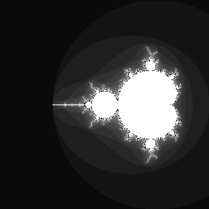
What you see is a Fractal, a highly fractured geometric picture, and more specifically one of the most famous representatives: the Mandelbrot Set. I am not familiar at all with the mathematics behind fractals, so I won't talk about them, or I will simply end up saying something wrong.

Such a highly featured and attractive picture is obtained from a really simple algorithm. It can be explained easily: take a grid of points on the plane, like for example a simple sheet of graph paper. Choose a scale for the axes. For every point (x,y) of the plane now do the following:

1. start with an empty vector (a,b) containing (0.0, 0.0)
2. create a new (a,b) vector as (a^2^ - b^2^ + x, 2ab
   • y)
3. continue with the procedure given in 2. If the length of the vector (a,b) becomes larger than 2.0, plot the (x,y) point black or a shade of gray, depending how far you got in the iterations. Instead, if the length of the vector stays below 2.0 after a given maximum amount of iterations, plot the (x,y) point white.

This, as said, decides the color of one single point (hence, a pixel of the image). Repeat for all the pixels and what you obtain is the Mandelbrot set.

You can also think in terms of complex numbers, plotting on the complex plane. Instead of (a,b) we now have a single complex number z~*0*~, and instead of (x,y) we now have a complex number c. The repeated operation now can be described as

1. z~*0*~ = 0.0
2. c = current complex number expressed by the current pixel point on the complex plane
3. repeatedly compute*z*~*n*+1~ = z~*n*~^2^
   • c
4. if the absolute value of*z* goes beyond 2.0, plot black or gray, otherwise plot white, as given before.

What if you change the starting point? What if we choose z~*0*~ = 1.0 instead of 0.0, or z~*0*~ = 1.0 i ? I tinkered with the program a bit. Here are the results. This image shows how the Mandelbrot Set changes when z~*0*~ goes from -3 to 3 (step 0.1). The set "blows away" towards the left, when going either towards -3 or +3.

If you change z~*0*~ along the imaginary axis, going from -3.0 i to 3.0 i, what you obtain is instead:

It blows away towards the right. So I said, what happens if I increase both the real part and the imaginary part together? will they "balance out" ? Not really. It burns away

I have absolutely no idea of what all this means from the strict mathematical point of view, except the fact that I am exploring the space of the values of z~*0*~ and how the Mandelbrot changes accordingly. I thought it was just cool to try it out.